Introduction

The transformer is a sequence-to-sequence neural architecture that revolutionized natural language processing by efficiently learning contextual representations through parallelized attention mechanisms. Originally introduced for machine translation in the seminal paper “Attention is All you Need” by Vaswani et al. (2017) , transformers have since become the foundation for most modern NLP systems.

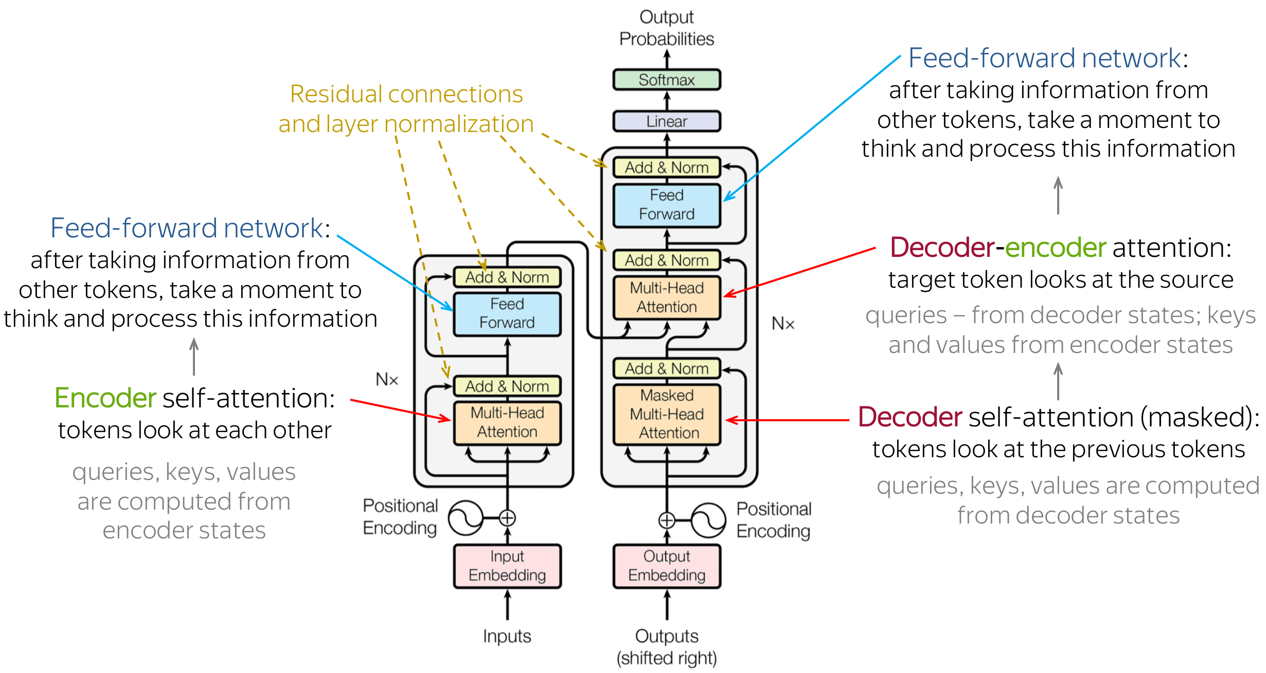
Figure 1. Overview of the Transformer Architecture (Source).

Transformers process sequential data (e.g., language), and excel at tasks where understanding the relationships between elements in the sequence is important. For example:

Machine Translation: Automatically converts text from one language to another.

Input: English sentence
Output: Same sentence in French
Text Summarization: Produces a concise summary from a longer piece of text.

Input: Long article
Output: Short summary
Text Generation: Generates new text based on a given prompt or partial sentence.

Input: Prompt or partial sentence
Output: Continuation or full sentence
Question Answering: Finds or generates answers to questions based on a provided passage.

Input: Passage and a question
Output: Answer extracted or generated from the passage
Text Classification: Assigns predefined categories or labels to a given text based on its content.

Input: Product review
Output: Sentiment label (e.g., positive, negative)

Motivation

The motivation behind the transformer architecture stems from the limitations of earlier sequence-to-sequence models based on Recurrent Neural Networks (RNNs).

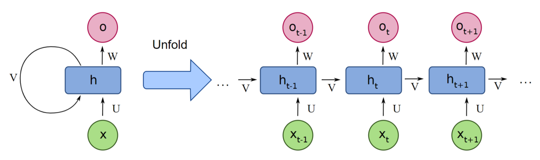
RNNs process sequences step-by-step, one token at a time. At each time step, the input token $x_t$ passes through the network, producing two outputs: an output token $o_t$ and a state vector $h_t$. For the next time step, the following input token $x_{t+1}$ is processed together with the previous state vector $h_t$, which is updated to $h_{t+1}$. The state vector carries context from previous steps, allowing the model to retain information from earlier tokens as it processes each new token. However, with each new input, the state vector is slightly changed, causing the model to gradually lose information about earlier context in long sequences. It is as if the model had to “free up space” from previous iterations to be able to store information from more recent tokens.

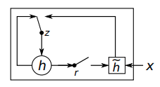
Figure 2. Recurrent Neural Network (RNN): At each time step $t$, the RNN receives an input token $x_t$ along with a state vector $h_{t-1}$, and produces an output token $o_t$ as well as an updated state vector $h_t$. This recurrent process allows the model to maintain contextual information across the sequence. Source: Raj, Dinesh Samuel Sathia et al.

Other variations of RNNs attempt to mitigate this issue. For example, Gated Recurrent Units (GRUs) use gating mechanisms to control the flow of information by deciding when and how much to update the state vector at each time step. This enables the model to retain relevant context over longer sequences by allowing it to ignore less important states.

Figure 3. Gated Recurrent Units (GRUs): The update gate $z$ determines how much of the previous hidden state $h_{t-1}$ is carried forward versus how much is updated with the new candidate hidden state $\tilde{h}_t$. The reset gate $r$ controls how much of the previous hidden state is ignored when computing the candidate hidden state. Source: Cho, Kyunghyun, et al.

Although these mechanisms help, the fundamental architectural issues associated with sequential processing still persist:

Information loss over long contexts: For long sequences, the state vector gradually loses information from earlier time steps, which are overwritten by information from later time steps.
Compute inefficiency due to non-parallelizable operations: To generate a token $o_t$ at time step $t$, all previous inputs $x_i$ for $i < t$ must be processed sequentially. This lack of parallelism makes computation extremely inefficient when training on extremely large models and datasets.

Core Concept: Self-Attention

The core component powering the transformer architecture is the Self-Attention (SA) mechanism. Instead of relying on a state vector that is countinuously updated at each time step, self-attention allows every token in the sequence to “attend” to (i.e., be influenced by) all other tokens directly, in parallel. This means that any token $x_t$ can consider the context of all tokens $x_i$ (for all $i$) simultaneously. This overcomes the information loss over long contexts that occurs in RNNs.

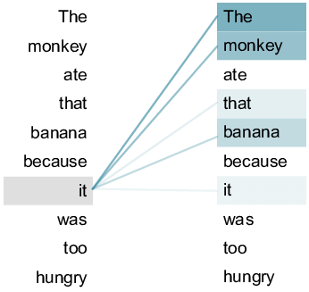
Figure 4. The token "it" attends to all other tokens in the sequence simultaneously. Attenion scores between the token "it" and the tokens "The", "monkey", "that", "banana", "it" are high. Source: Huiqiang Xie, Zhijin Qin, Geoffrey Li (2021).

Additionally, because attention is computed in parallel across the entire sequence using highly efficient matrix operations, modern hardware such as GPUs and TPUs can be leveraged to greatly accelerate both training and inference, enabling training larger models on bigger datasets.

This solves the two major shortcomings of RNNs that we’ve discussed previously.

However, this design shift in the architecture from RNNs to self-attention, does not come only with benefits. The self-attention mechanism has important drawbacks in comparison to RNNs:

Quadratic computational complexity: For a sequence of length $N$, this requires computing an $N{\times}N$ attention matrix. This leads to a computational and memory complexity of $O(N^2)$, i.e., doubling the input length quadruples the necessary computation. In contrast, RNNs have a linear complexity of $O(N)$, i.e., doubling the input length also doubles the necessary computation. This quadratic scaling makes processing very long sequences expensive.
Fixed-size sequence length: A direct consequence of the quadratic complexity is that Self-Attention must operate on a fixed-length context window. All input sequences are truncated or padded to a predefined maximum length (e.g., 512 tokens). This prevents the model from processing sequences of arbitrary length, a task that RNNs can handle naturally due to their step-by-step processing.

The Self-Attention mechanism is the core of the Transformer architecture, but other components are essential for it to function properly. Next, we will discuss each component in greater detail.

Components

The Transformer model is composed of several key components, each playing a crucial role in its functionality. These components include Word Embeddings and Positional Encodings, Self-Attention (SA), Multi-Head Self-Attention (MHA), Feed Forward Networks (FFN), Layer Normalization, and Residual Connections. Together, they enable the model to process input sequences, capture contextual relationships, and generate meaningful outputs. We’ll explore each of these components in detail to understand their purpose and implementation.

Word Embeddings and Positional Encodings

Unstructured inputs such as text or images must be converted into numerical representations before they can be processed by machine learning models. These numerical representations should encode information about the input in such a way that, for example, vectors representing two synonymous words are close together in the embedding space. There are several methods to learn such vectors. For example, Mikolov et al. (2013) introduced the continuous bag-of-words and continuous skip-gram models, which learn dense, low-dimensional vectors that capture the semantic meaning of words.

Figure 5. Word Embeddings (Source).

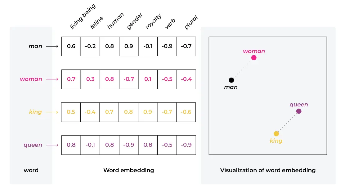
With transformers, input tokens are mapped into dense vectors using an embedding layer. The embedding matrix is initialized randomly with shape (vocabulary_size, embedding_dimension) and is learned jointly with the rest of the model during training. Each input token retrieves its corresponding embedding from this table, providing a continuous vector representation that captures semantic properties of the token.

Along with word embeddings, the transformer architecture introduces a second type of embedding called positional encodings. This is necessary because the self-attention mechanism is invariant to the order of tokens in the input sequence. Since self-attention processes all tokens in parallel, it treats the input as a set rather than a sequence. Without positional information, the model cannot distinguish between the first, second, or any other position in the sequence, and thus cannot capture the sequential structure of language.

To address this, we introduce positional encodings that explicitly encode the order of tokens. There are two main approaches to computing positional encodings: using sinusoidal functions or learning the positional encodings jointly with the model. Each method has its own advantages and drawbacks, and the choice often depends on the specific application and requirements.

Sinusoidal positional encodings (as introduced in the original Transformer paper) use fixed sine and cosine functions of different frequencies to encode each position. This approach allows the model to extrapolate to sequence lengths not seen during training and provides a deterministic, non-learnable way to represent position.
Learned positional encodings treat the positional embeddings as parameters that are learned during training, similar to word embeddings. This approach allows the model to adapt the positional information to the specific dataset and task, potentially improving performance, but may not generalize as well to longer sequences.

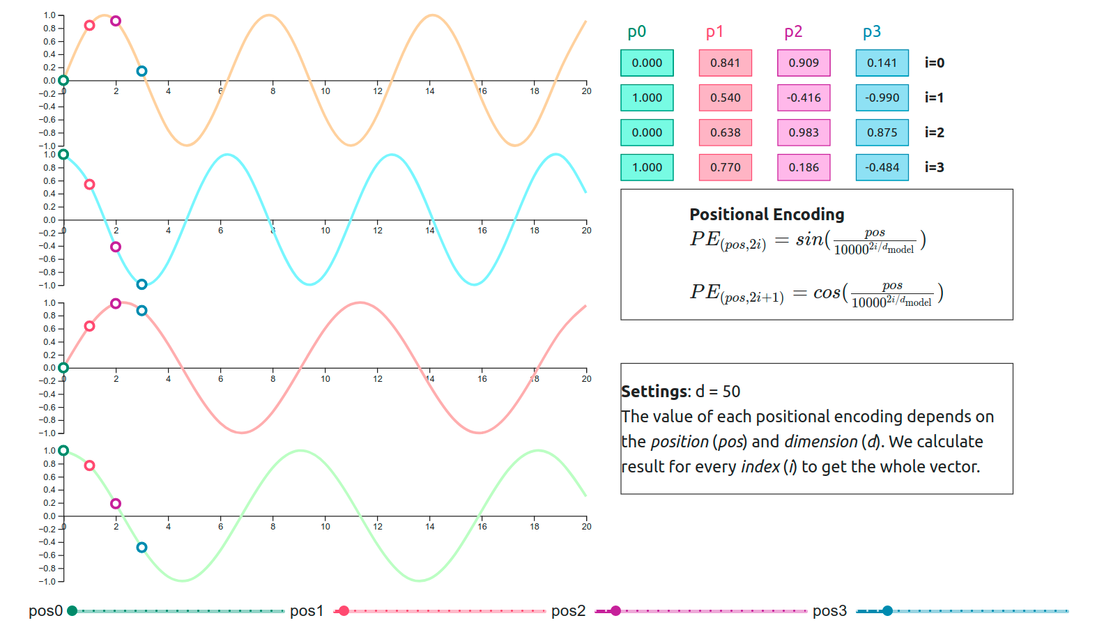
Figure 6. Sinusoidal positional encodings (Source).

The final input to the transformer block is the element-wise sum of the word embeddings and the positional encodings, allowing the model to capture both semantic meaning and positional information.

Note that the input to the embedding layer is a sequence of token ids, and the output is a matrix of size (context_window, embedding_dimension), where each row represents an input token, and each column represents a feature.

Implementation

The implementation below considers the approach of jointly learning the positional encodings alongside the rest of the model components.

class EmbeddingLayer(nn.Module):
    def __init__(self, vocab_size, embedding_dim, context_length):
        super().__init__()
        self.word_embedding_layer = nn.Embedding(vocab_size, embedding_dim)
        self.positional_encoding_layer = nn.Embedding(context_length, embedding_dim)

        self.register_buffer("positions", torch.arange(context_length))

    def forward(self, x):
        word_emb = self.word_embedding_layer(x)
        pos_emb = self.positional_encoding_layer(self.positions)

        return word_emb + pos_emb

Self-Attention (SA)

The goal of the self-attention mechanism is to transform each input token’s static embeddings into contextual embeddings that incorporate the semantics of other tokens in the sequence. As discussed previously, SA achieves this by allowing any token in the input sequence to influence any other token directly, allowing the model to capture dependencies regardless of their distance in the sequence. (see Figure 4).

Example: Static vs. Contextual Embeddings

Suppose the input token is “bat”. Its static embedding might encode general characteristics such as: “is an animal”, “is associated with flying”, and “is a nocturnal creature”. This embedding remains unchanged regardless of context.

Now consider the same token “bat” in the context of this sentence:

“He swung the bat and hit a home run.”

Here, the surrounding tokens “swung”, “hit”, and “home run” provide context that shifts the meaning of “bat”. Through self-attention, the contextual embedding for “bat” will incorporate features like: “is a piece of sports equipment”, “is used in baseball”, and “is something to swing and hit a ball”

Now, the contextual vector for “bat” reflects the specific meaning in the context of this sentence, which is defined by the other tokens in the sentence.

Note that in order to determine the contextual meaning of “bat” in the sentence, this token needs to identify two things:

Which tokens in the sequence are most relevant to me?

How much information from each token should I incorporate?

Implementing Self-Attention

Each token’s static embedding will be transformed into three different vectors: query, key, and value. They can be interpreted in the following manner:

Query: What features am I searching for in other tokens? (What am I looking for?)
Key: What features do I present to other tokens, so they can determine if I am relevant to them? (How do I describe myself to others?)
Value: What information do I carry that should be shared if another token attends to me? (What do I represent?)

We define three weight matrices (i.e., linear layers): Key ($W_K$), Query ($W_Q$), and Value ($W_V$). Each of these matrices will multiply the input sentence embedding matrix to obtain $Q$, $K$, and $V$.

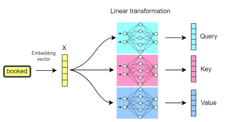
Figure 7. Keys, Queries, and Values: Three randomly initialized matrices multiply the input embedding to obtain the Keys, Queries, and Values for that particular input sequence (Source).

Now to obtain the contextual embeddings, we apply the following equation:

\[\begin{equation}\text{Attention}(Q, K, V) = \text{softmax}\left(\frac{QK^T}{\sqrt{d_k}}\right) V\end{equation}\]

Let’s break the equation down step-by-step.

Dot Product ($QK^T$)

Let’s ignore the term $\sqrt{d_k}$ for now. Remember the intuitive meaning of $Q$ (What am I looking for?) and $K$ (How do I describe myself to others?). When we perform a dot-product between $Q$ and $K^T$, we are essentially computing a similarity score between the two features. If ${Q_i}K^T_j$ is high, it means that token $j$ has the kind of features that token $i$ is looking for. Let’s illustrate this with an example.

Imagine we have three tokens from the sentence “The cats are chasing the mouse”: chasing, cat, and mouse. For the self-attention mechanism, each token generates Query, Key, and Value vectors. Here, we’ll focus on how chasing computes attention scores with respect to cat and mouse.

Let’s assume the following Query and Key vectors have been generated:

$Q_{chasing} = [-2.0, \ 3.0, \ 2.5, \ -1.0, \ 1.5, \ -2.0]$
$K_{cat} = [-1.8, \ 2.8, \ 3.0, \ 0.2, \ 2.5, \ -1.5]$
$K_{mouse} = [-1.5, \ -2.0, \ 2.8, \ -0.5, \ -2.0, \ 3.0]$

1. Score: chasing → cat

We compute the dot product of the query from chasing and the key from cat.

$Q_{chasing} \cdot K_{cat} = [-2.0, 3.0, 2.5, -1.0, 1.5, -2.0] \cdot [-1.8, 2.8, 3.0, 0.2, 2.5, -1.5]$

The step-by-step multiplication of corresponding elements looks like this:

$(-2.0 \times -1.8) = 3.6$ (Match ✅)
$(3.0 \times 2.8) = 8.4$ (Strong Match ✅)
$(2.5 \times 3.0) = 7.5$ (Strong Match ✅)
$(-1.0 \times 0.2) = -0.2$ (Minor Mismatch ❌)
$(1.5 \times 2.5) = 3.75$ (Match ✅)
$(-2.0 \times -1.5) = 3.0$ (Match ✅)

The final similarity score is the sum of these products: $3.6 + 8.4 + 7.5 - 0.2 + 3.75 + 3.0 = \textbf{26.05}$

2. Score: chasing → mouse

Next, we compute the dot product of the query from chasing and the key from mouse.

$Q_{chasing} \cdot K_{mouse} = [-2.0, 3.0, 2.5, -1.0, 1.5, -2.0] \cdot [-1.5, -2.0, 2.8, -0.5, -2.0, 3.0]$

The step-by-step multiplication reveals significant disagreement:

$(-2.0 \times -1.5) = 3.0$ (Match ✅)
$(3.0 \times -2.0) = -6.0$ (Strong Mismatch ❌)
$(2.5 \times 2.8) = 7.0$ (Strong Match ✅)
$(-1.0 \times -0.5) = 0.5$ (Minor Match ✅)
$(1.5 \times -2.0) = -3.0$ (Mismatch ❌)
$(-2.0 \times 3.0) = -6.0$ (Strong Mismatch ❌)

The final similarity score reflects this poor alignment: $3.0 - 6.0 + 7.0 + 0.5 - 3.0 - 6.0 = \textbf{-4.5}$

The high positive score for cat and the negative score for mouse indicate that “cat” is far more relevant to “chasing” in this context.

Let’s continue on to the next part of the equation.

Softmax

The Softmax function transforms the raw attention scores (ranging from $-\infty$ to $+\infty$) into a normalized probability distribution over all tokens in the sequence. Each score is exponentiated and divided by the sum of all exponentiated scores, resulting in values between $0$ and $1$ that sum to $1$. This ensures that the most relevant tokens receive higher weights, while less relevant tokens are assigned lower weights, allowing the model to focus its attention appropriately.

Figure 8. Softmax (Source).

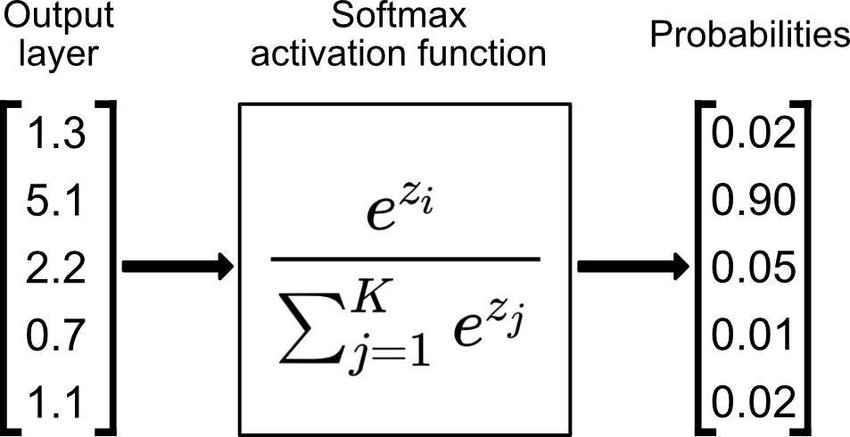
Note that the softmax functions does exactly what its name suggests: a soft version of a max function. With a max function, we would get a $1$ for the largest element in the sequence, and $0$ for everything else. With softmax, we want the highest values to accumulate most of the probability mass, with smaller values being close to $0$.

The Scaling Factor ($\sqrt{d_k}$)

The reason to introduce the scaling factor $\sqrt{d_k}$ is because of how the dot product and the softmax function behave. Dot products can grow large, especially with high-dimensional vectors. Large inputs can push the Softmax function into regions where its gradient is almost zero, which makes training unstable. The scaling term $\sqrt{d_k}$ (where $d_k$ is the dimension of $K$) mitigates this issue by ensuring the input to the softmax function is not extremely large.

Attention Scores

What we’ve computed so far, $softmax\left(\frac{QK^T}{\sqrt{d_k}}\right)$, gives us the attention scores in the form of a square matrix of size $N{\times}N$, where $N$ is the sequence length, and each entry in the matrix represents how much attention token $i$ should pay to token $j$, i.e., how relevant token $j$ is to token $i$ in this particular sentence.

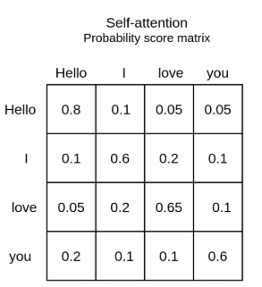
Figure 9: Attention scores for an input sequence "Hello I love you". (Source)

Final Step: Computing the Contextual Vectors

Now the only thing left is to multiply the attention scores by $V$, which contains the actual information of a token that we want to aggregate (remember, $V$ -> What do I represent?):

\[Z_i = \sum_{j} \text{Attention}(i, j) \cdot V_j\]

Note that $Z_i$, the contextual embedding for token $i$, is composed of all the $V_j$ vectors for every token $j$ in the sequence, weighted by how much they are important to token $i$.

(Optional) Self-Attention as a Soft Hash Table

Another good example to build intuition for how the Self-Attention mechanism works is to compare it with the concept of a lookup table / hash table / dictionary.

In a python dictionary, a query will either match entirely with an existing key (and then return its value), or it will not match at all with any of the keys (and then return an error or a predefined value):

d = {
    "dog": "bark",
    "wolf": "howl",
    "cat": "meow"
}

# this key exists, the query will match and return "bark"
query1 = "dog" 
value1 = lookup[query1]

print(value1)
### Output: "bark"

# this query doesnt match with any existing key, and we will get an error
query2 =  "bird"
value2 = lookup[query2]

print(value2)
### Output: Exception

In the attention mechanism, we are performing a similar operation, but we implement a “soft” match of keys and queries. In fact, all queries will match will all keys, but in different intensities. The softmax computation introduces this notion of intensity, which will weigh the value that is returned.

d = {
    "dog": "bark":,
    "wolf": "howl",
    "cat": "meow"
}

# query doesn't exist in the dictionary
query = "husky"

# but we can compute its similarity with the existing keys
# assume that the 'similarity' and 'softmax' functions exist.
similarities = [similarity(key, query) for key in d.keys()]
attention_scores = [softmax(s/sqrt(d_k)) for s in similarities]
contextual_vector = [
    attn_score * value for attn_score, value in zip(attention_scores, d.values())
]

# example:
# similarities = [4.0, 3.0, -1.0]
# attention_scores = [0.70, 0.26, 0.04]  
# contextual_vector = [0.70 * "bark", 0.26 * "howl", 0.04 * "meow"]

# this now represents the token that is associated with the query "husky"

Masked Self-Attention

In tasks involving sequence generation (e.g., language modeling), it is important that the model does not have access to future tokens when predicting the current token. For example, consider the sentence:

“The cat sat on the mat.”

When generating this sequence, the model should predict each word one at a time, without seeing the words that come after. When predicting “sat”, the model can only use “The cat” as context, not “on the mat”. If the model could see future tokens, it could simply copy them, making the task trivial and preventing it from learning meaningful language patterns.

To “blind” the model from accessing future tokens, we use masked self-attention. In practice, we apply a mask to the attention matrix, setting the attention scores for future positions to $-\infty$ before applying softmax, which will set the weight of these tokens to $0$. As a result, any token $x_i$ can only use information from itself and previous tokens $x_j$ with $j \leq i$.

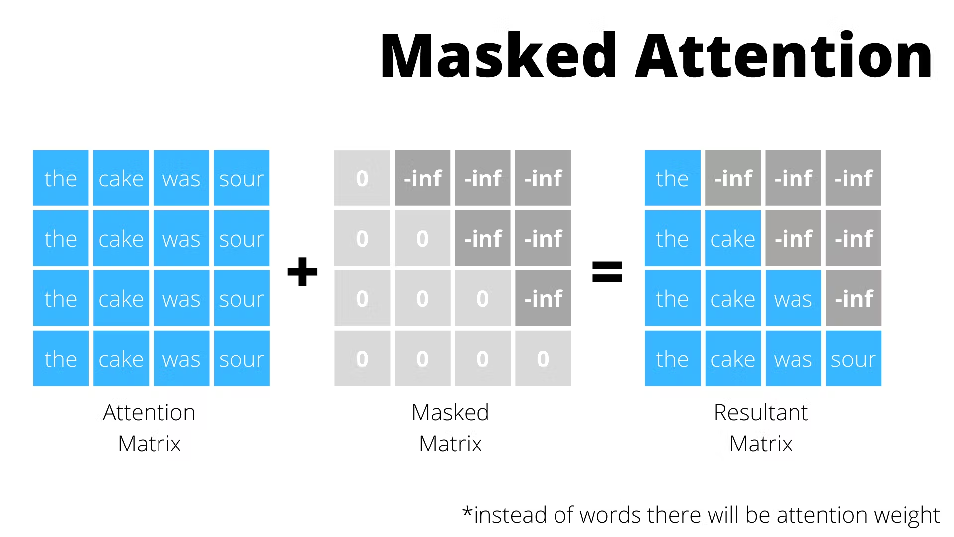
Figure 6. Attention Matrix Masking (Source).

We’ll revisit the details of encoder and decoder blocks later, but for now, note that masked self-attention is only used in the decoder.

Implementation

This implementation of SA can be used with and without a mask, depending on the parameter mask set on the forward method.

class AttentionHeadLayer(nn.Module):
    def __init__(self, embedding_dim, head_size, context_window):
        super().__init__()
        self.head_size = head_size
        self.w_k = nn.Linear(embedding_dim, head_size, bias=False)
        self.w_q = nn.Linear(embedding_dim, head_size, bias=False)
        self.w_v = nn.Linear(embedding_dim, head_size, bias=False)

        # create an upper triangular matrix with boolean values
        # [[False, True, True],
        # [False, False, True],
        # [False, False, False]]
        triu_mask = torch.triu(
            torch.ones(context_window, context_window), diagonal=1
        ).to(torch.bool)

        self.register_buffer("mask", triu_mask)
        self.embedding_dim = embedding_dim

    def forward(self, x, mask=False):
        batch_size, window_size, emb_size = x.size()

        k = self.w_k(x)
        v = self.w_v(x)
        q = self.w_q(x)

        z = self.compute_contextual_vector(k, q, v, mask)

        return z

    def compute_contextual_vector(self, k, q, v, mask=False):
        matmul = einops.einsum(
            q,
            k,
            "batch len_q head, batch len_k head -> batch len_q len_k"
        )
        if mask:
            matmul = torch.masked_fill(matmul, self.mask, -torch.inf)

        attn_scores = nn.functional.softmax(matmul / self.embedding_dim**0.5, dim=-1)

        contextual_vectors = einops.einsum(
            attn_scores,
            v,
            "batch ctx_len_i ctx_len_j, batch ctx_len_i head -> batch ctx_len_j head"
        )
        return contextual_vectors

Multi-Head Self-Attention (MHA)

Transformers use Multi-Head Self-Attention (MHA) instead of a single self-attention unit. MHA enables the model to capture a richer set of relationships and patterns in the input sequence by running several attention operations in parallel. This allows the model to focus on different aspects of the input simultaneously.

For example, in a sentence like “The cat sat on the mat,” one attention head might focus on syntactic relationships, such as identifying that “cat” is the subject of “sat,” while another head might focus on semantic relationships, such as associating “mat” with its spatial connection to “sat.”

The practical difference between a single self-attention unit and MHA lies in how the input embeddings are processed. In MHA, the input embedding is passed through multiple self-attention units in parallel. For instance, if we have an MHA with 4 self-attention units, each unit will output a contextual vector whose dimension is $1/4$ of the final contextual vector. These smaller contextual vectors are then concatenated to form the final contextual vector.

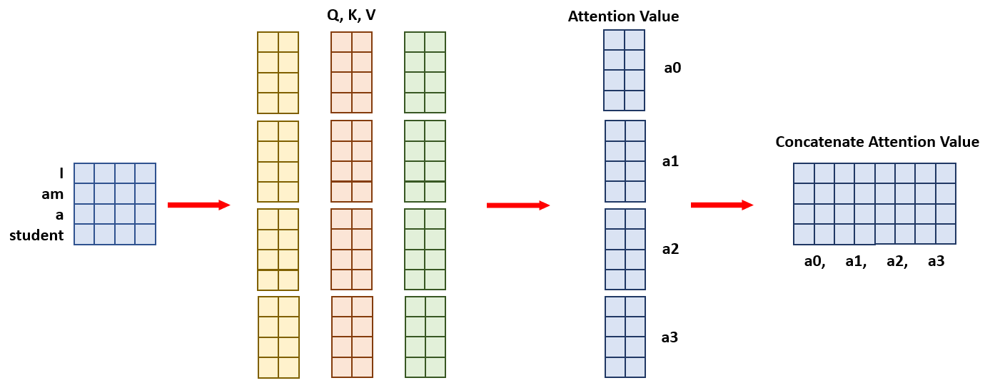
Figure 7. Multi-Head Self-Attention (MHA): Input sequence "I am a student" is processed through $4$ SA units with embedding_dim equals $2$. The attention values $a_0, a_1, a_2, a_3$ are concatenated to form the output with embedding_dim equals $8$ (Source).

To ensure that the features from different heads are not confined to specific sections of the concatenated vector, this combined output is passed through a linear layer. This enables the model to learn how to combine the diverse information captured by each attention head, creating a more cohesive representation.

Implementation

class MultiHeadAttentionLayer(nn.Module):
    def __init__(self, embedding_dim, n_heads, context_window):
        super().__init__()

        head_dim = embedding_dim // n_heads

        self.attn_head_list = nn.ModuleList(
            AttentionHeadLayer(
                embedding_dim,
                head_dim,
                context_window
            ) for _ in range(n_heads)
        )
        self.ff_layer = nn.Linear(embedding_dim, embedding_dim)

    def forward(self, x, mask=False):
        out = torch.cat(
            [attn_head(x, mask=mask) for attn_head in self.attn_head_list], dim=-1
        )
        out = self.ff_layer(out)

        return out

Point-Wise Feed Forward Network (FFN)

Up to now, all operations performed are linear transformations (e.g., matrix multiplications). Linear functions are those where the output grows proportionately to the input. For example, in a function like $y = 2x$, doubling the input $x$ will double the output $y$.

Although we are performing several of these operations sequentially, the combination of multiple linear operations remains linear.

However, most real-world problems involve non-linear relationships that cannot be captured by linear transformations alone, such as:

Exponentials: $y = 2^x$, doubling the input quadruples the output.
Quadratics: $y = x^2$, doubling the input increases the output by a factor of four.
Sinusoids: $y = \sin(x)$, where the output oscillates periodically and does not grow linearly with the input.
Logarithms: $y = \log(x)$, where the output grows slower as the input increases.
Piecewise Functions: $y = \begin{cases} x & \text{if } x < 0 \\ x^2 & \text{if } x \geq 0 \end{cases}$, where the behavior changes depending on the input range.
Step Functions: $y = \text{step}(x)$, where the output jumps abruptly at certain input values.

By introducing non-linear activation functions such as ReLU, sigmoid, or tanh, the model can capture non-linear relationships, enabling it to approximate more complex mappings between inputs and outputs.

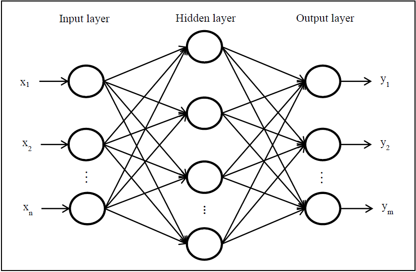
To introduce non-linearity, we use a point-wise feed forward network with a non-linear activation function, such as ReLU, applied after the MHA layer.

This consists of two linear layers that perform an up projection followed by a down projection, meaning the input gets stretched to a higher dimensional space, then gets down projected to the original size after leaving the hidden unit.

Figure 8. Point-Wise Feed Forward Network: Input gets up projected from $3$ to $4$ dimensions, then down projected back from $4$ to $3$ dimensions. Source: Garg, Siddhant & Ramakrishnan, Goutham. (2020) .

Implementation

class PointWiseFFNLayer(nn.Module):
    def __init__(self, dim_embedding):
        super().__init__()

        self.net = nn.Sequential(
            nn.Linear(dim_embedding, dim_embedding*4),
            nn.ReLU(),
            nn.Linear(dim_embedding*4, dim_embedding),
        )

    def forward(self, x):
        out = self.net(x)

        return out

Layer Normalization

Layer normalization is a procedure that helps stabilise and accelerate the training process by reducing internal covariate shift. Internal covariate shift means the distribution of inputs to a layer changes during training as the parameters of the previous layers are updated.

Suppose the first layer outputs values with a mean of $0$ and a variance of $1$ at the start of training. After a few optimization steps, the outputs shift to have a mean of $5$ and a variance of $10$. The second layer, which was initially trained to expect inputs centered around $0$ with a small variance, now receives inputs that are drastically different. This forces the second layer to adapt its weights, slowing down training and destabilizing the optimization process.

Layer normalization addresses this issue by normalizing the outputs of the layers so that their distribution have a mean of $0$ and a variance of $1$. It also learns two parameters $\gamma$ and $\beta$ to scale and shift the distribution if needed. This is a key engineering component in ensuring that large and deep neural networks can converge in a stable fashion.

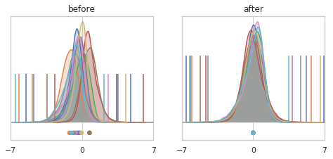
Figure 9. Before layer normalization, the activations exhibit significantly varying distributions. After normalization, the distributions are aligned and much closer to each other (Source).

To normalize the input features, we scale them as follows:

\[\hat{x}_i = \frac{x_i - \mu_i}{\sqrt{\sigma_i^2 + \epsilon}}\]

Where:

$x_i$ is the $i$-th feature for input $x$.
$\mu_i$ is the mean of the input features for the $i$-th dimension.
$\sigma_i^2$ is the variance of the input features for the $i$-th dimension.
$\epsilon$ is a small constant added for numerical stability.
$\hat{x}_i$ is the normalized feature for the $i$-th dimension.

After normalization, the output is scaled and shifted using learnable parameters $\gamma$ (scale) and $\beta$ (shift):

\[y_i = \gamma \hat{x}_i + \beta\]

This ensures that the model can learn to adjust the normalized values as needed.

Implementation

class LayerNorm(nn.Module):
    def __init__(self, embedding_dim):
        super().__init__()

        self.gamma = nn.Parameter(torch.ones(embedding_dim))
        self.beta = nn.Parameter(torch.zeros(embedding_dim))

        self.eps = 1e-5

    def forward(self, x):
        mean = x.mean(dim=-1, keepdim=True)
        var = x.var(dim=-1, keepdim=True, unbiased=False)

        
        norm_x = (x-mean) / (var**2 + self.eps)**1/2
        scaled_shifted_x = self.gamma * norm_x + self.beta

        return scaled_shifted_x

Residual Connections

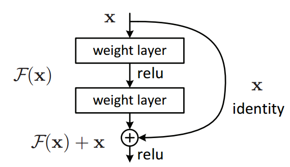
Residual connections were introduced by He et al. (2015) to address the problem of vanishing gradients.

When updating weights, the gradients are multiplied by the weights of each layer. If these weights are small (i.e., close to zero), the gradients shrink as they propagate backward through many layers, eventually approaching zero, which makes earlier layers effectively stop learning.

Residual connections help mitigate this problem by allowing gradients to bypass layers, preserving their magnitude. This is done simply by summing the input of a given layer with its output.

Figure 11: Residual Connection in a feed forward neural network. The input $X$ branches in two directions: the first direction goes into the layer and is processed normally. The other direction skips the layer completely, (i.e., the input is not changed at all). Both branches are aggregated afterwards. Source: He, Kaiming, et al. (2016) .

Implementation

class GenericLayer(nn.Module):
    def __init__(self):
        super().__init__()
        self.net = nn.Sequential(
            ...
        )

    def forward(self, x):
        out = x + self.net(x)

        return out

Full Implementation with Practical Example

Check this google collab to test the architecture with a practical example borrowed from Andrej Karpathy’s lecture series.

class EmbeddingLayer(nn.Module):
    def __init__(self, vocab_size, embedding_dim, context_length):
        super().__init__()
        self.word_embedding_layer = nn.Embedding(vocab_size, embedding_dim)
        self.positional_encoding_layer = nn.Embedding(context_length, embedding_dim)

        self.context_length = context_length
        self.register_buffer("positions", torch.arange(self.context_length))

    def forward(self, x):
        word_emb = self.word_embedding_layer(x)
        pos_emb = self.positional_encoding_layer(self.positions)

        return word_emb + pos_emb

class AttentionHeadLayer(nn.Module):
    def __init__(self, embedding_dim, head_size, context_window):
        super().__init__()
        self.head_size = head_size
        self.w_k = nn.Linear(embedding_dim, head_size, bias=False)
        self.w_q = nn.Linear(embedding_dim, head_size, bias=False)
        self.w_v = nn.Linear(embedding_dim, head_size, bias=False)

        self.register_buffer("mask", torch.triu(torch.ones(context_window, context_window), diagonal=1).to(torch.bool))
        self.embedding_dim = embedding_dim

    def forward(self, x, mask=False):
        batch_size, window_size, emb_size = x.size()

        k = self.w_k(x)
        v = self.w_v(x)
        q = self.w_q(x)

        z = self.compute_contextual_vector(k, q, v, mask)

        return z

    def compute_contextual_vector(self, k, q, v, mask=False):
        # Q @ K.T -> i j k @ i m k -> i j m
        matmul = einops.einsum(q, k, "batch len_q head, batch len_k head -> batch len_q len_k")
        if mask:
            matmul = torch.masked_fill(matmul, self.mask, -torch.inf)

        attn_scores = nn.functional.softmax(matmul / self.embedding_dim**0.5, dim=-1)

        # attn_scores @ v -> i j m x i j k -> i m k
        contextual_vectors = einops.einsum(
            attn_scores,
            v,
            "batch ctx_len_i ctx_len_j, batch ctx_len_i head -> batch ctx_len_j head"
        )
        return contextual_vectors

class MultiHeadAttentionLayer(nn.Module):
    def __init__(self, embedding_dim, n_heads, context_window):
        super().__init__()

        head_dim = embedding_dim // n_heads

        self.attn_head_list = nn.ModuleList(
            AttentionHeadLayer(embedding_dim, head_dim, context_window) for _ in range(n_heads)
        )
        self.ff_layer = nn.Linear(embedding_dim, embedding_dim)

    def forward(self, x, mask=False):
        out = torch.cat([attn_head(x, mask=mask) for attn_head in self.attn_head_list], dim=-1)
        out = self.ff_layer(out)

        return out

class FeedForwardLayer(nn.Module):
    def __init__(self, dim_embedding):
        super().__init__()

        self.net = nn.Sequential(
            nn.Linear(dim_embedding, dim_embedding*2),
            nn.ReLU(),
            nn.Linear(dim_embedding*2, dim_embedding),
        )

    def forward(self, x):
        out = self.net(x)

        return out

class LayerNormLayer(nn.Module):
    def __init__(self, embedding_dim):
        super().__init__()

        self.layernorm = nn.LayerNorm(embedding_dim)

    def forward(self, x):
        out = self.layernorm(x)

        return out

class DecoderBlock(nn.Module):
    def __init__(self, embedding_dim, n_attn_heads, context_window):
        super().__init__()

        self.mha_layer = MultiHeadAttentionLayer(embedding_dim, n_attn_heads, context_window)
        self.layernorm_mha = LayerNormLayer(embedding_dim)

        self.ffn_layer = FeedForwardLayer(dim_embedding)
        self.layernorm_ffn = LayerNormLayer(embedding_dim)
        self.dropout = nn.Dropout(0.1)


    def forward(self, x):
        norm_x = self.layernorm_mha(x)
        out = self.mha_layer(norm_x, mask=True)
        x = x + self.dropout(out)

        norm_x = self.layernorm_ffn(x)
        out = self.ffn_layer(norm_x)
        x = x + self.dropout(out)

        return out

class CLFHead(nn.Module):
    def __init__(self, embedding_dim, vocab_size):
        super().__init__()

        self.clf_head = nn.Linear(embedding_dim, vocab_size)

    def forward(self, x):
        out = self.clf_head(x)

        return out

class DecoderTransformer(nn.Module):
    def __init__(self, vocab_size, context_length, embedding_dim, n_attn_heads, num_trf_blocks):
        super().__init__()

        self.emb_layer = EmbeddingLayer(vocab_size, embedding_dim, context_length)
        self.trf_blocks = nn.Sequential(
            *[DecoderBlock(
                embedding_dim,
                n_attn_heads,
                context_length) for _ in range(num_trf_blocks)
            ]
        )
        self.clf_head = CLFHead(embedding_dim, vocab_size)

    def forward(self, x, y=None):
        out = self.emb_layer(x)
        out = self.trf_blocks(out)
        out = self.clf_head(out)

        loss = None
        if y is not None:
            # This rearranging is needed because pytorch's CE loss expects a 2D vector for logits
            out = einops.rearrange(out, "b t c -> (b t) c")
            y = einops.rearrange(y, "b t -> (b t)")
            loss = nn.functional.cross_entropy(out, y)

        return out, loss

    def generate(self, idx, max_new_tokens):
        for _ in range(max_new_tokens):
            idx_cond = idx[:, -block_size:]
            logits, _ = self(idx_cond)
            logits = logits[:, -1, :]
            probs = F.softmax(logits, dim=-1)
            idx_next = torch.multinomial(probs, num_samples=1)
            idx = torch.cat((idx, idx_next), dim=1)
        return idx

Architecture Variations

In this post I’ve only discussed the decoder-only transformer architecture. A brief presentation of the other variations can be found below.

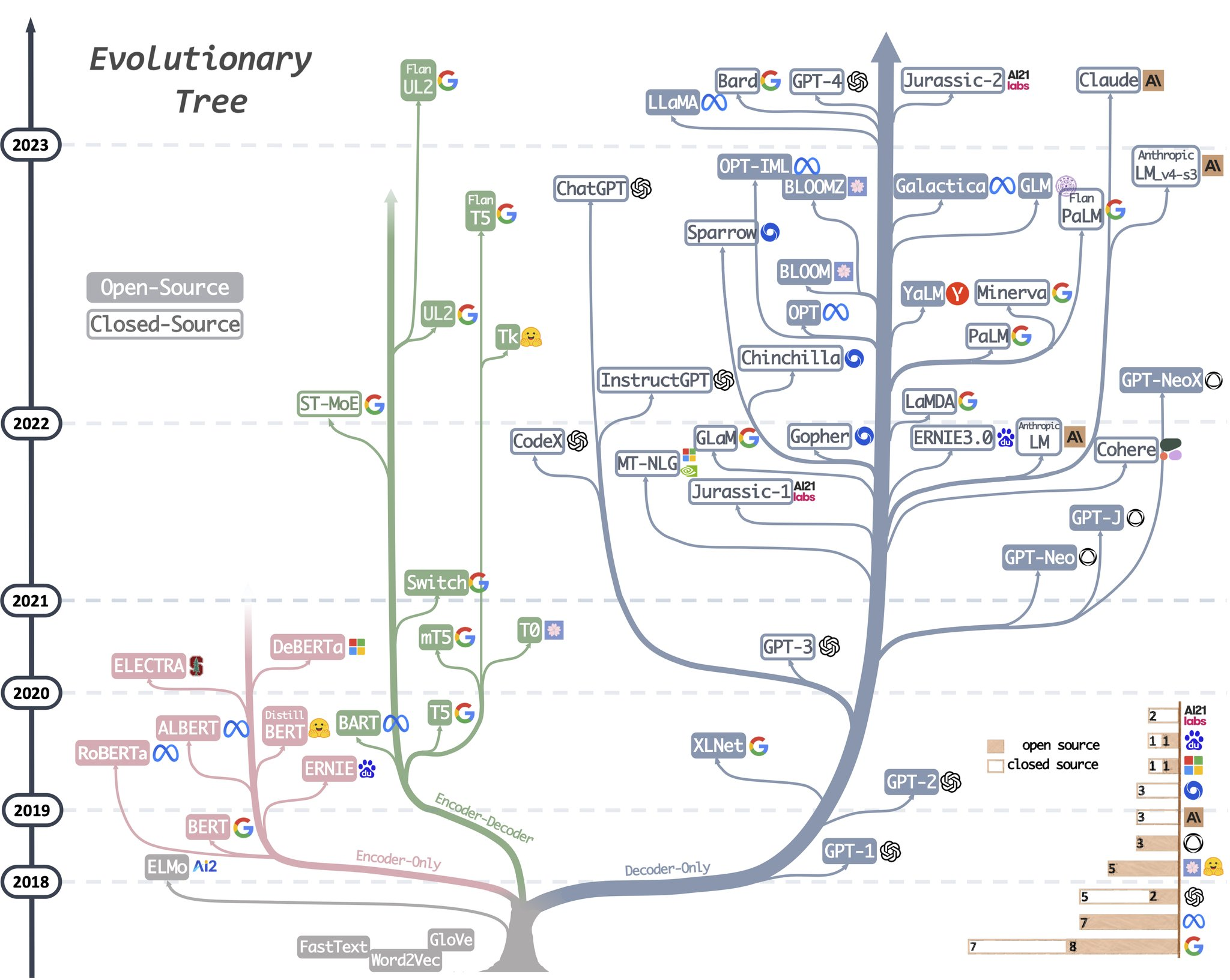
Figure 12: Evolutionary Tree of Language Models (Source).

Encoder-Decoder (suitable for seq2seq tasks)

Suitable for sequence-to-sequence tasks such as machine translation, text summarisation, image captioning.
Encoder-Decoder models have the advantage of bidirectionality when calculating the attention scores. In other words, the encoder’s MHA is not masked, allowing tokens from time any step to attend to ALL tokens (from past and future time steps) instead of only the past tokens as in the decoder.
In general terms, the model is allowed to process the input entire sequence first (e.g., such as a sentence in English), and then it will generate the output tokens (e.g., such as a translation of the input sentence to German) one token at a time.
Examples of Encoder-Decoder models: BART, T5, T0
One important implementation detail about encoder-decoder architectures that was not mentioned previously, is that the second MHA layer in the decoder takes the Key and the Value outputs from the encoder as input, while the Query comes from the Masked MHA from the decoder (refer to the first figure).

Encoder-only (suitable for input understanding tasks e.g. classification)

Encoder-only architectures are suitable for classification tasks, since we don’t want to map the input sequence to another sequence, but rather map the input sequence to a pre-defined set of labels. Therefore, we only need to encode, i.e., learn how to represent the sequence in latent space, and then append a classification head on top to discriminate between the classes. Common tasks using encoder-only models include: text classification, named entity recognition (NER), question answering (with extractive approaches), document embeddings.
Encoder-only models also have bidirectionality, and are simpler and more efficient than encoder-decoder models. However, they are not suitable for generative tasks, as they only encode the sequence, but can’t decode it.
Examples of encoder-only models: BERT, RoBERTa, DeBERTa

Decoder-only (suitable for generative tasks)

Decoder-only architectures are suitable for generative tasks, since these settings are naturally autoregressive (dependant on previous context).
Tasks suitable for decoder-only models include: language modelling, text generation, dialogue systems, text autocompletion.
Examples of decoder-only models: XLNeT, GPT-3, ChatGPT, LLaMa.

References

Vaswani, A. et al. (2017). Attention Is All You Need.
Raj, D. S. et al. (2019). Analysis of Big Data Technology for Health Care Services.
Chung, J. et al. (2014). Empirical Evaluation of Gated Recurrent Neural Networks on Sequence Modeling.
Cho, K. et al. (2014). Learning Phrase Representations Using RNN Encoder–Decoder for Statistical Machine Translation.
Xie, H. et al. (2021). Deep Learning Enabled Semantic Communication Systems.
Mikolov, T. et al. (2013). Efficient Estimation of Word Representations in Vector Space.
Garg, S. and Ramakrishnan, G. (2020). Advances in Quantum Deep Learning: An Overview.
He, K. et al. (2016). Deep Residual Learning for Image Recognition.